38 how to add horizontal labels in excel graph

How to add a line in Excel graph: average line, benchmark, etc. Switch to the Marker section, expand Marker Options, change it to Built-in, select the horizontal bar in the Type box, and set the Size corresponding to the width of your bars (24 in our example): Set the marker Fill to Solid fill or Pattern fill and select the color of your choosing. Excel Horizontal Bar Graph Data Label Adjustment Create a 3rd column for Data Labels and enter the following formula: =B2&" "&TEXT (C2,"0%") B2 is the N cell & C2 is the % cell Then drag it down till the last label Once done, add data label from value from cells and select the cells from the newly created column Hope this was useful! Report abuse Was this reply helpful? Yes No BL BlakeG_184

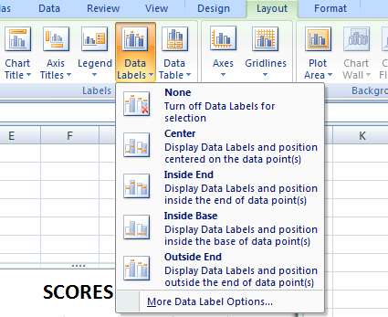
How to add or move data labels in Excel chart? - ExtendOffice To add or move data labels in a chart, you can do as below steps: In Excel 2013 or 2016. 1. Click the chart to show the Chart Elements button . 2. Then click the Chart Elements, and check Data Labels, then you can click the arrow to choose an option about the data labels in the sub menu. See screenshot: In Excel 2010 or 2007

How to add horizontal labels in excel graph

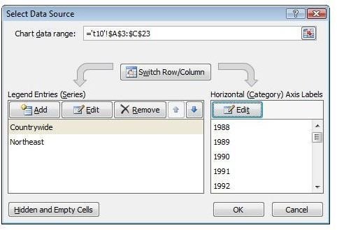
Excel charts: add title, customize chart axis, legend and data labels To add a chart title in Excel 2010 and earlier versions, execute the following steps. Click anywhere within your Excel graph to activate the Chart Tools tabs on the ribbon. On the Layout tab, click Chart Title > Above Chart or Centered Overlay. Link the chart title to some cell on the worksheet › charts › add-data-pointAdd Data Points to Existing Chart – Excel & Google Sheets Start with your Graph. Similar to Excel, create a line graph based on the first two columns (Months & Items Sold) Right click on graph; Select Data Range . 3. Select Add Series. 4. Click box for Select a Data Range. 5. Highlight new column and click OK. Final Graph with Single Data Point Excel tutorial: How to customize axis labels You won't find controls for overwriting text labels in the Format Task pane. Instead you'll need to open up the Select Data window. Here you'll see the horizontal axis labels listed on the right. Click the edit button to access the label range. It's not obvious, but you can type arbitrary labels separated with commas in this field.

How to add horizontal labels in excel graph. How to Label Axes in Excel: 6 Steps (with Pictures) - wikiHow Select the graph. Click your graph to select it. 3 Click +. It's to the right of the top-right corner of the graph. This will open a drop-down menu. 4 Click the Axis Titles checkbox. It's near the top of the drop-down menu. Doing so checks the Axis Titles box and places text boxes next to the vertical axis and below the horizontal axis. Add a Horizontal Line to an Excel Chart - Peltier Tech When the Paste Special dialog appears, make sure you select these options: Add Cells as a New Series, Y Values in Columns, Series Names in First Row, Categories (X Values) in First Column. Click OK and the new series will appear in the chart. Add a Horizontal Line to a Column or Line Chart Change the scale of the horizontal (category) axis in a chart On the Format tab, in the Current Selection group, click the arrow in the box at the top, and then click Horizontal (Category) Axis. On the Format tab, in the Current Selection group, click Format Selection. In the Format Axis pane, do any of the following: How to Add Axis Titles in Excel - YouTube In previous tutorials, you could see how to create different types of graphs. Now, we'll carry on improving this line graph and we'll have a look at how to a...

HOW TO CREATE A BAR CHART WITH LABELS INSIDE BARS IN EXCEL - simplexCT 7. In the chart, right-click the Series "# Footballers" Data Labels and then, on the short-cut menu, click Format Data Labels. 8. In the Format Data Labels pane, under Label Options selected, set the Label Position to Inside End. 9. Next, in the chart, select the Series 2 Data Labels and then set the Label Position to Inside Base. How to add a horizontal line to the chart - Microsoft Excel 365 E.g., this will be useful to show data with some goal line or limits: To add a horizontal line to your chart, do the following: 1. Add the cell or cells with the goal or limit (limits) to your data, for example: 2. Add a new data series to your chart by doing one of the following: How to Add Axis Labels in Excel Charts - Step-by-Step (2022) - Spreadsheeto How to add axis titles 1. Left-click the Excel chart. 2. Click the plus button in the upper right corner of the chart. 3. Click Axis Titles to put a checkmark in the axis title checkbox. This will display axis titles. 4. Click the added axis title text box to write your axis label. How To Add Axis Labels In Excel - BSUPERIOR Add Title one of your chart axes according to Method 1 or Method 2. Select the Axis Title. (picture 6) Picture 4- Select the axis title. Click in the Formula Bar and enter =. Select the cell that shows the axis label. (in this example we select X-axis) Press Enter. Picture 5- Link the chart axis name to the text.

› Make-a-Bar-Graph-in-ExcelHow to Make a Bar Graph in Excel: 9 Steps (with Pictures) May 02, 2022 · Customize your graph's appearance. Once you decide on a graph format, you can use the "Design" section near the top of the Excel window to select a different template, change the colors used, or change the graph type entirely. The "Design" window only appears when your graph is selected. To select your graph, click it. support.microsoft.com › en-us › officeAdd or remove titles in a chart - support.microsoft.com Under Labels, click Axis Titles, point to the axis that you want to add titles to, and then click the option that you want. Select the text in the Axis Title box, and then type an axis title. To format the title, select the text in the title box, and then on the Home tab, under Font , select the formatting that you want. How to Change Horizontal Axis Labels in Excel | How to Create Custom X ... Download the featured file here: this video I explain how to chang... How to Change Horizontal Axis Values - Excel & Google Sheets Right click on the graph. Select Data Range. 3. Click on the box under X-Axis. 4. Click on the Box to Select a data range. 5. Highlight the new range that you would like for the X Axis Series. Click OK.

Excel Help: Making Pyramid Graph for Headcount Distribution Representation

Excel Graph - horizontal axis labels not showing properly Open your Excel file Right-click on the sheet tab Choose "View Code" Press CTRL-M Select the downloaded file and import Close the VBA editor Select the cells with the confidential data Press Alt-F8 Choose the macro Anonymize Click Run Upload it on OneDrive (or an other Online File Hoster of your choice) and post the download link here.

Best Excel Tutorial - Slope Graph

Use text as horizontal labels in Excel scatter plot Edit each data label individually, type a = character and click the cell that has the corresponding text. This process can be automated with the free XY Chart Labeler add-in. Excel 2013 and newer has the option to include "Value from cells" in the data label dialog. Format the data labels to your preferences and hide the original x axis labels.

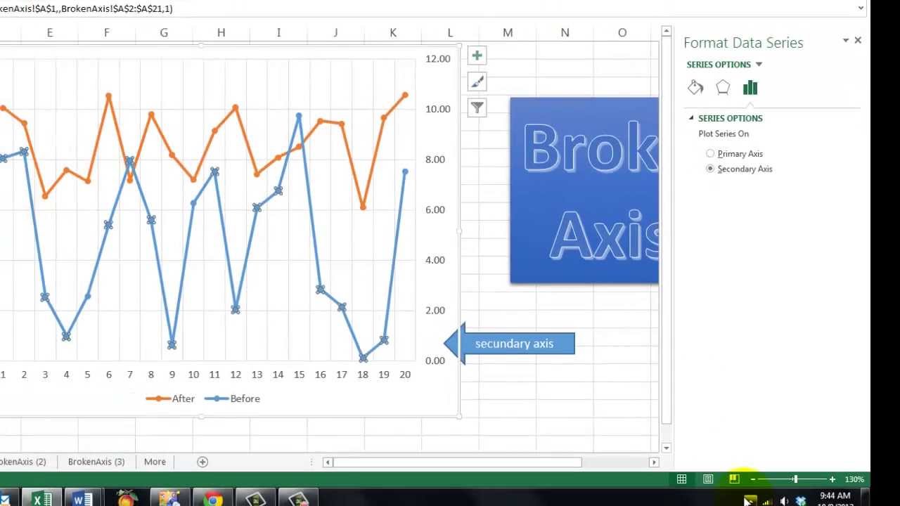
Does Excel Have a Broken Axis? - YouTube

Add / Move Data Labels in Charts - Excel & Google Sheets Adding Data Labels Click on the graph Select + Sign in the top right of the graph Check Data Labels Change Position of Data Labels Click on the arrow next to Data Labels to change the position of where the labels are in relation to the bar chart Final Graph with Data Labels

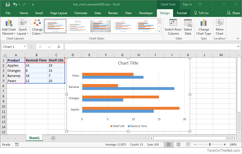
MS Office Suit Expert : MS Excel 2016: How to Create a Bar Chart

How to add axis label to chart in Excel? - ExtendOffice If you are using Excel 2010/2007, you can insert the axis label into the chart with following steps: 1. Select the chart that you want to add axis label. 2. Navigate to Chart Tools Layout tab, and then click Axis Titles, see screenshot: 3. You can insert the horizontal axis label by clicking Primary ...

How to add data labels to a Column (Vertical Bar) Graph in Microsoft® Excel 2013 - YouTube

› Add-a-Graph-to-Microsoft-WordHow to Add a Graph to Microsoft Word: 11 Steps ... - wikiHow Jul 28, 2022 · Click a cell in the Excel window. Doing so will select it, which will allow you to add a point of data to that cell. The values in the "A" column dictate the X-axis data of your graph. The values in the "1" row each pertain to a different line or bar (e.g., "B1" is a line or bar, "C1" is a different line or bar, and so on).

Create a line chart with bands [tutorial] | Chandoo.org - Learn Microsoft Excel Online

How to add extra axis labels in a logarithmic chart in Excel 2010? Right-click on your chart > Select Data > Add a new series > call it "Axis Labels", and add the series X and Y values from your version of the above table. 4. Move the mouse until you find one of your "Axis Labels" data points on the chart just outside (to the left) of the graph area, and right click. If you do this correctly, you can then see ...

how to add data labels into Excel graphs — storytelling with data

Excel tutorial: How to create a multi level axis To straighten out the labels, I need to restructure the data. First, I'll sort by region and then by activity. Next, I'll remove the extra, unneeded entries from the region column. The goal is to create an outline that reflects what you want to see in the axis labels. Now you can see we have a multi level category axis.

How to Data Labels in a Line Graph in Excel 2010 - YouTube

Add or remove data labels in a chart - support.microsoft.com Add data labels to a chart Click the data series or chart. To label one data point, after clicking the series, click that data point. In the upper right corner, next to the chart, click Add Chart Element > Data Labels. To change the location, click the arrow, and choose an option.

how to make a excel graph.

› article › bar-graph-in-excelBar Graph in Excel — All 4 Types Explained Easily Bar Graph in Excel — All 4 Types Explained Easily (Excel Sheet Included) Note: This guide on how to make a bar graph in Excel is suitable for all Excel versions. Bar graphs are one of the most simple yet powerful visual tools in Excel. Bar graphs are very similar to column charts, except that the bars are aligned horizontally. Related:

Excel Version 16 For Mac Adding Graph Labels - fasrtune

How to Add a Horizontal Line in a Chart in Excel - Excel Champs Next step is to change that average bars into a horizontal line. For this, select the average column bar and Go to → Design → Type → Change Chart Type. Once you click on change chart type option, you'll get a dialog box for formatting. Change the chart type of average from "Column Chart" to "Line Chart With Marker". Click OK.

Text Labels on a Vertical Column Chart in Excel - Peltier Tech Blog

How to Insert Axis Labels In An Excel Chart | Excelchat We will go to Chart Design and select Add Chart Element. Figure 3 - How to label axes in Excel. In the drop-down menu, we will click on Axis Titles, and subsequently, select Primary Horizontal. Figure 4 - How to add excel horizontal axis labels. Now, we can enter the name we want for the primary horizontal axis label.

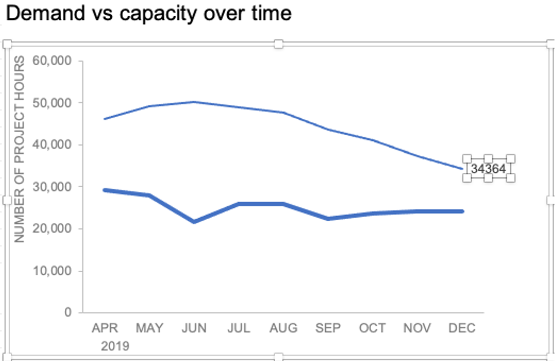
storytelling with data: plotting a value within a range

excelchamps.com › excel-charts › people-graphHow to Insert a People Graph in Excel | 7 Steps | Info ... Jul 05, 2017 · In a people graph, instead of a column, bar, or line, we have icons to present the data. And, it looks nice and professional. Today, in this post, I’d like to share simple steps to insert a people graph in Excel and the option which we can use with it. So let’s get started. 7 Steps to Insert a People Graph in Excel

How to Change Labels for a Chart Axis in Excel 2007

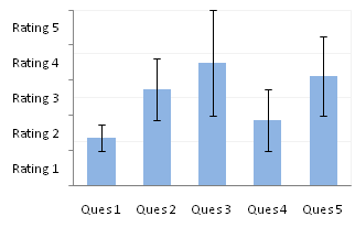
Text Labels on a Horizontal Bar Chart in Excel - Peltier Tech On the Excel 2007 Chart Tools > Layout tab, click Axes, then Secondary Horizontal Axis, then Show Left to Right Axis. Now the chart has four axes. We want the Rating labels at the bottom of the chart, and we'll place the numerical axis at the top before we hide it. In turn, select the left and right vertical axes.

How to Label Axes in Excel: 6 Steps (with Pictures) - wikiHow

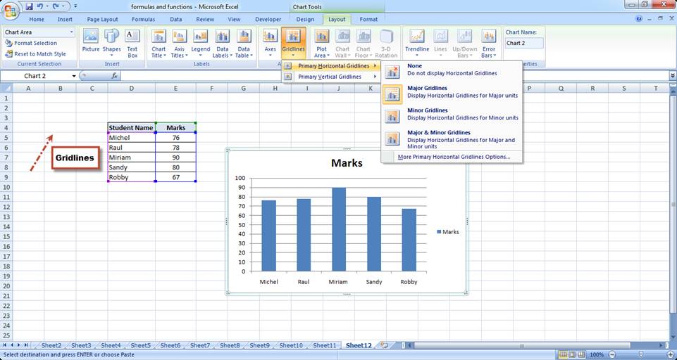
spreadsheetplanet.com › add-gridlines-in-chart-excelHow to Add Gridlines in a Chart in Excel? 2 Easy Ways! Let us now see two ways to insert major and minor gridlines in Excel. Method 1: Using the Chart Elements Button to Add and Format Gridlines The Chart Elements button appears to the right of your chart when it is selected. This button allows you to add, change or remove chart elements like the title, legend, gridlines, and labels.

How to label graphs in Excel | Think Outside The Slide

How to Add Axis Titles in a Microsoft Excel Chart - How-To Geek Add Axis Titles to a Chart in Excel. Select your chart and then head to the Chart Design tab that displays. Click the Add Chart Element drop-down arrow and move your cursor to Axis Titles. In the pop-out menu, select "Primary Horizontal," "Primary Vertical," or both. If you're using Excel on Windows, you can also use the Chart ...

Excel - 2-D Bar Chart - Change horizontal axis labels - Super User

"how to add horizontal axis label in excel graph" Veja aqui Curas Caseiras, Mesinhas, sobre How to add horizontal axis label in excel graph. Descubra as melhores solu es para a sua patologia com Todos os Beneficios da Natureza Outros Remédios Relacionados: how To Add Horizontal Axis Labels In Excel Chart; how To Add X Axis Label In Excel Chart; how To Add X Axis Label In Excel Graph

Changing X-Axis Values - YouTube

Excel tutorial: How to customize axis labels You won't find controls for overwriting text labels in the Format Task pane. Instead you'll need to open up the Select Data window. Here you'll see the horizontal axis labels listed on the right. Click the edit button to access the label range. It's not obvious, but you can type arbitrary labels separated with commas in this field.

Basic Excel Chart Formatting - MS Excel Charting Tutorial Part 4 | Vertical Horizons

› charts › add-data-pointAdd Data Points to Existing Chart – Excel & Google Sheets Start with your Graph. Similar to Excel, create a line graph based on the first two columns (Months & Items Sold) Right click on graph; Select Data Range . 3. Select Add Series. 4. Click box for Select a Data Range. 5. Highlight new column and click OK. Final Graph with Single Data Point

Share :